Quantum Monte Carlo is used in quantum mechanics to understand the electronic structure of molecular and solid state systems. MiniQMC, like QMCPACK, implements a direct solve of the Schrodinger wave equation, which provides accuracy at the expense of computational intensity. From the wave equation, the probability of particle position and particle energy are computed. MiniQMC and QMCPACK both implement Variational and Diffusion Monte Carlo (DMC). DMC samples the exact wave function, where Variational Monte Carlo (VMC) uses an approximate wave function. In this work, we focus on DMC.
This is the pseudocode for DMC in miniQMC: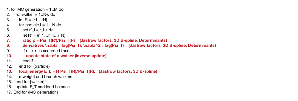
Each walker represents a 3D particle position, R. An ensemble of walkers
is generationally and stochastically propagated through a defined
electronic structure. Each propagation step moves the particle through
the structure using a drift-diffusion process. The particle’s local energy
is computed at each step to determine if the particle dies, continues
propagation, or reproduces. This changing particle population potentially
creates imbalance that is addressed by periodic load balancing.
The lines shown in bold red in the figure are the most computationally
and/or memory intensive steps in the algorithm. These are associated with
key kernels. The four key kernels in both miniQMC and QMCPACK are the
following:
- Determinant update (inverse update): This kernel uses the
Sherman-Morrison algorithm to compute the Slater determinant. The
Slater determinant provides an accurate approximation of the wave
functions being solved. This kernel relies on BLAS2 functions and is
the source of the N3 scaling in the application. - Splines: This kernel is invoked for every potential electron move.
It computes the 3D spline value, the gradient (4×4×4×N stencil), and
the Laplacian of electron orbitals. This kernel is memory bandwidth
limited. Its large memory footprint makes data layout and memory
hierarchy considerations critical to performance. - Jastrow factors (1, 2, and 3-body): The Jastrow factor represents
the electronic correlation beyond the mean-field level in QMC
simulations. Correlations are decomposed into 1, 2, and 3-body terms
(electron-nucleus, electron-electron, and electron-electron-ion,
respectively). This is a computationally intensive kernel. - Distance tables: These tables hold distances between electrons and
electrons and atoms as matrices of all pairs of particle distances.
Two tables are maintained—one for electron-electron pairs and one
for electron-ion pairs. Minimum image and periodic boundary
conditions are applied. Tables are updated after every successful MC
electron move. Algorithms implementing this kernel have a strong
sensitivity to data layout.